2024 Presidential Election Analysis
Matthew E. Dardet, Harvard University
View the Project on GitHub matthewdardet/example-blog-jekyll
Introduction: Past Presidential Election Results
September 1, 2024
Predictions of the future are based on the patterns of the past. If X tended to predict Y well in the past, we would want to use that X in our model. So we start our journey by looking into past presidential election results – first at the national level.
Elections are generally competitive between the two parties. One thing in particular stands out: in the last 60 or so years, the race for the presidency has overall been remarkably competitive between the two major parties. Since FDR, neither Republicans nor Democrats have maintained a monopoly over the White House:
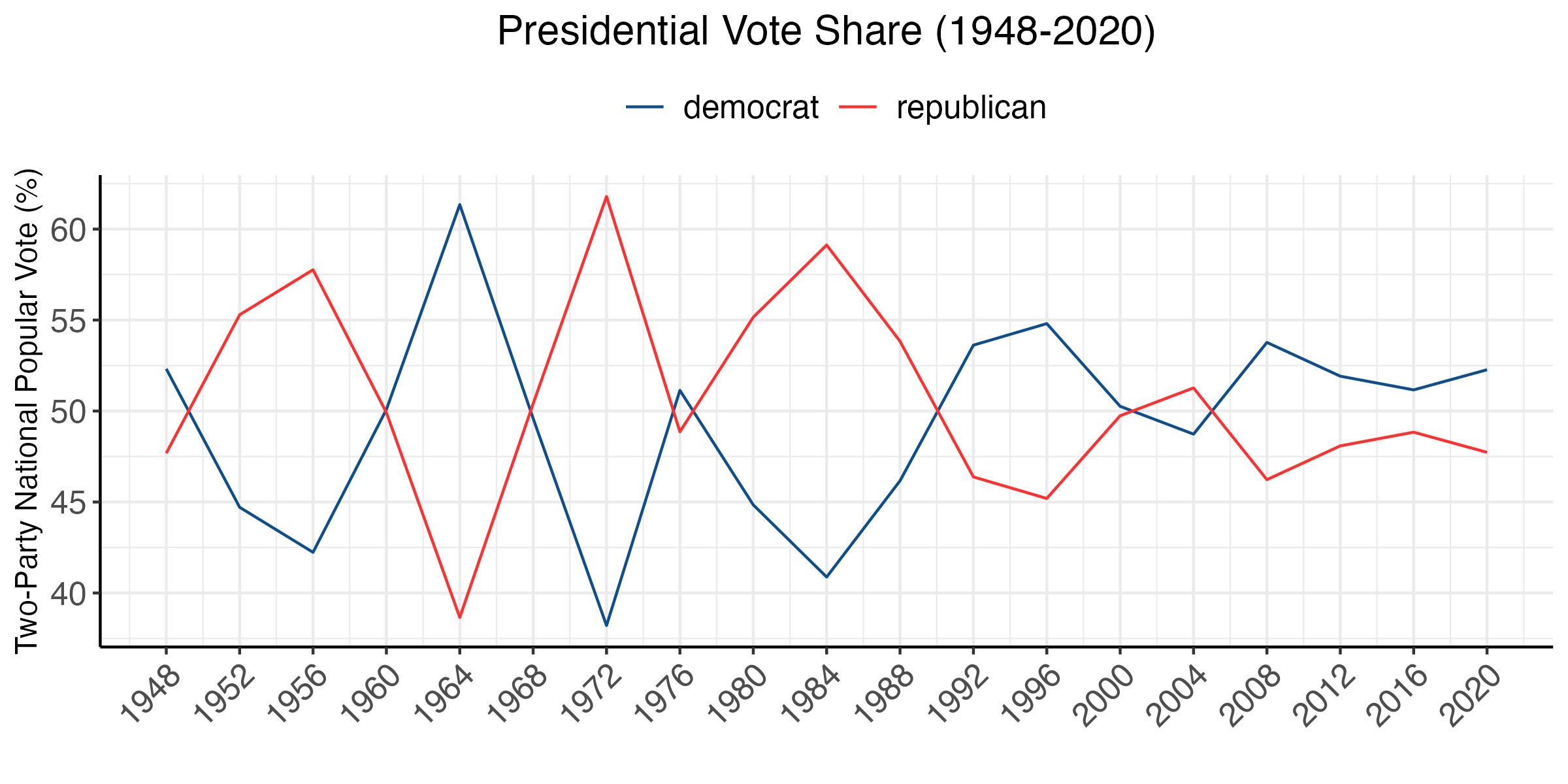
The first half of the twentieth century experienced greater swings and greater margins of victory, while point spreads in the last 20 years have been less than 10 points. The three closest elections in the last 60 years and their “prevailing narratives” are:
-
2000, margin of
0.5%or 500k votes or5 EV(Bush vs. Gore). Gore managed to distance himself from Clinton’s scandals (which put him neck-and-neck with Bush) though, really, this was anyone’s election. -
1968, margin of
0.7%or 500k votes or110 EV(Nixon vs. Humphrey). As the South began to realign, Nixon’s Southern Strategy appealed to whites in the South. Beginning of the “culture wars” which favored the Republicans in rural areas. Protests against Humphrey occurred due to his unpopular pro-war position. -
1960, margin of
0.7%or 120k votes or84 EV(JFK vs. Nixon). The Republican party was hurt by the 1958 recession (we’ll talk about this more when we read The Message Matters). JFK mobilized a new cohort of Catholic voters and campaigned wisely in key swing states.
Similarly, the three biggest landslides in the last 60 years and their “prevailing narratives” are:
-
1984, margin of
18.2%or 17 million votes or512 EV(Reagan vs. Mondale). Reagan was an effective speaker and campaigner who enjoyed a post-recession economic recovery and boom. -
1972, margin of
23.5%or 18 million votes or503 EV(Nixon vs. McGovern). The Republican party was helped by a strong economy and continued the Southern Strategy which massively appealed to a newly re-aligned South. McGovern was viewed by some as a radical and his VP’s bouts with depression were considered a scandal. -
1964, margin of
22.6%or 16 million votes or434 EV(Johnson vs. Goldwater). JFK’s assasination considered a shock sympathetic to Democrats. Despite the beginnings of racial realignment, Goldwater was portrayed as an extremist in media and campaigns. Johnson’s Great Society and civil rights reforms were enormous policy achievements.
We will explore this semester what empirical evidence we really have for these “prevailing narratives” and whether they generalize beyond these races.
A winner-take-all system with electors based on population distorts win margins. We note another set of observations around the winner’s popular vote. First, very famously in two races, the winner of the popular vote lost the election: Al Gore in 2000 and Hillary Clinton in 2016. This is a reflection of how each popular vote for a candidate is not equally valuable to their electoral victory because of the electoral college. The state where it is won matters.
For example, winning 25 million votes in California (a state with ~30 million voting-age citizens) is impressive but unnecessary to beat your opponent and win its 55 electoral votes (EV). Instead, it would be better if a candidate just won a slim majority of 15 million votes in California (55 EV), a slim majority of 5.1 million votes in Pennsylvannia (20 EV), and a slim majority of 4.5 million votes in North Carolina (15 EV). That’s the same 25 million votes, but in one scenario a candidate wins 55 EV while in the other a candidate wins 90 EV.
This is an illustration of the distortions of a winner-takes-all electoral system where slim majorities in just a few moderately large states (which promise substantial quantities of EVs) translate to huge electoral gains. Empirically, it ends up that electoral college vote margins are more dramatic than popular vote margins. This is why presidential candidates tend to (mostly) focus their resources on moderately large swing states where they can win by a slim majority rather than firing up the base or purusing lost causes.
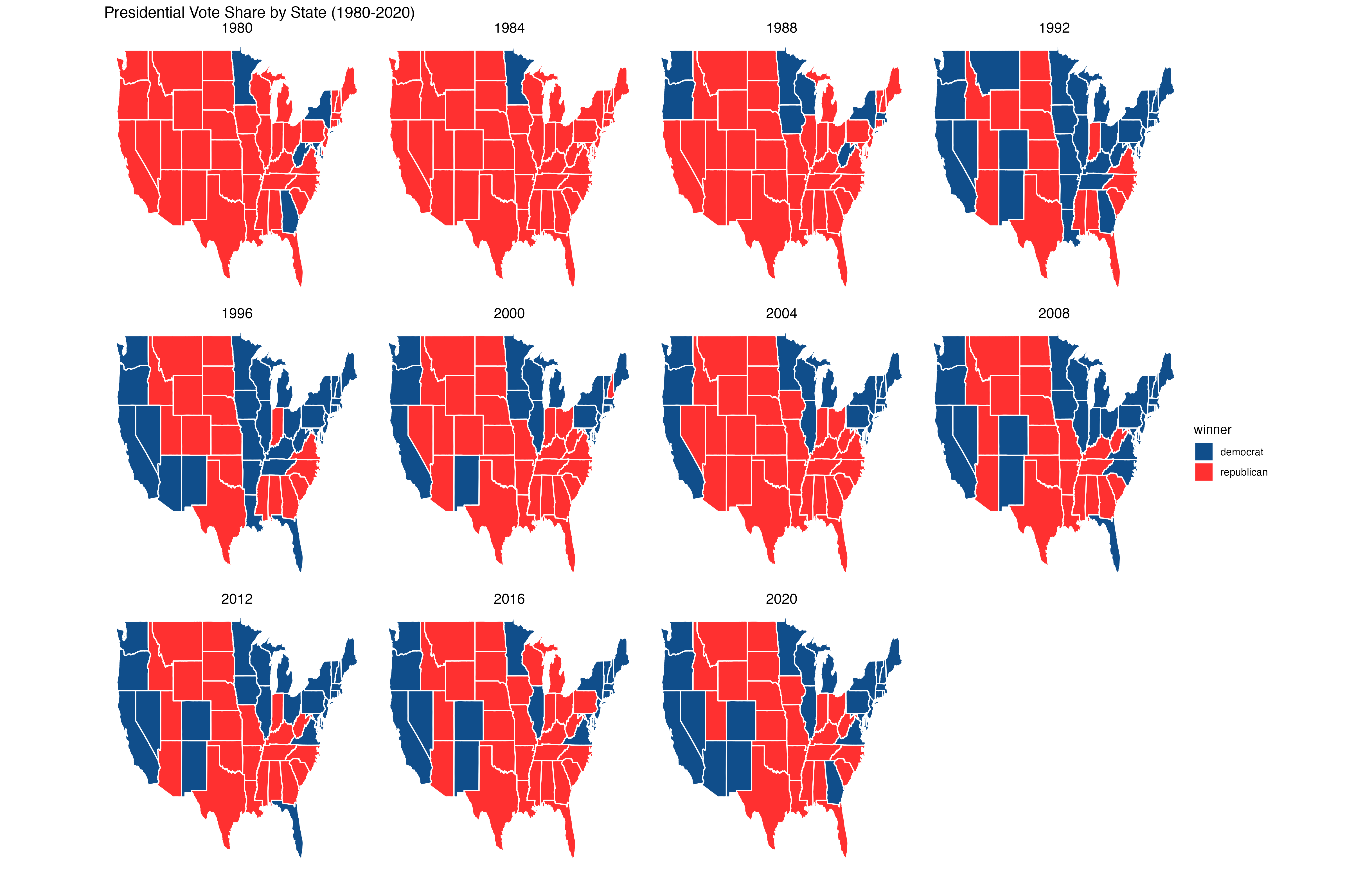
Below we can see which states vote blue/red and how consistently so. In section, we will produce more nuanced versions of these maps that highlight ‘‘swinginess’’ of various states.
Prediction 1: using past election returns. Noting from the first figure the general competitiveness of elections, we might infer that the best way to predict this year’s election in each state is looking at the two most recent electoral cycles. This is the simple but central engine of the Helmut Norpath electoral cycle model.
I will predict 2024 election state-by-state election outcomes, for each state i using a simplified version of this model by taking a weighted average of the past two election popular vote returns:
presvoteshare2024_i = (presvoteshare2020_i x 0.75) + (presvoteshare2016_i x 0.25)
See the related R script to replicate this analysis. The figure below shows the state-by-state forecasts:
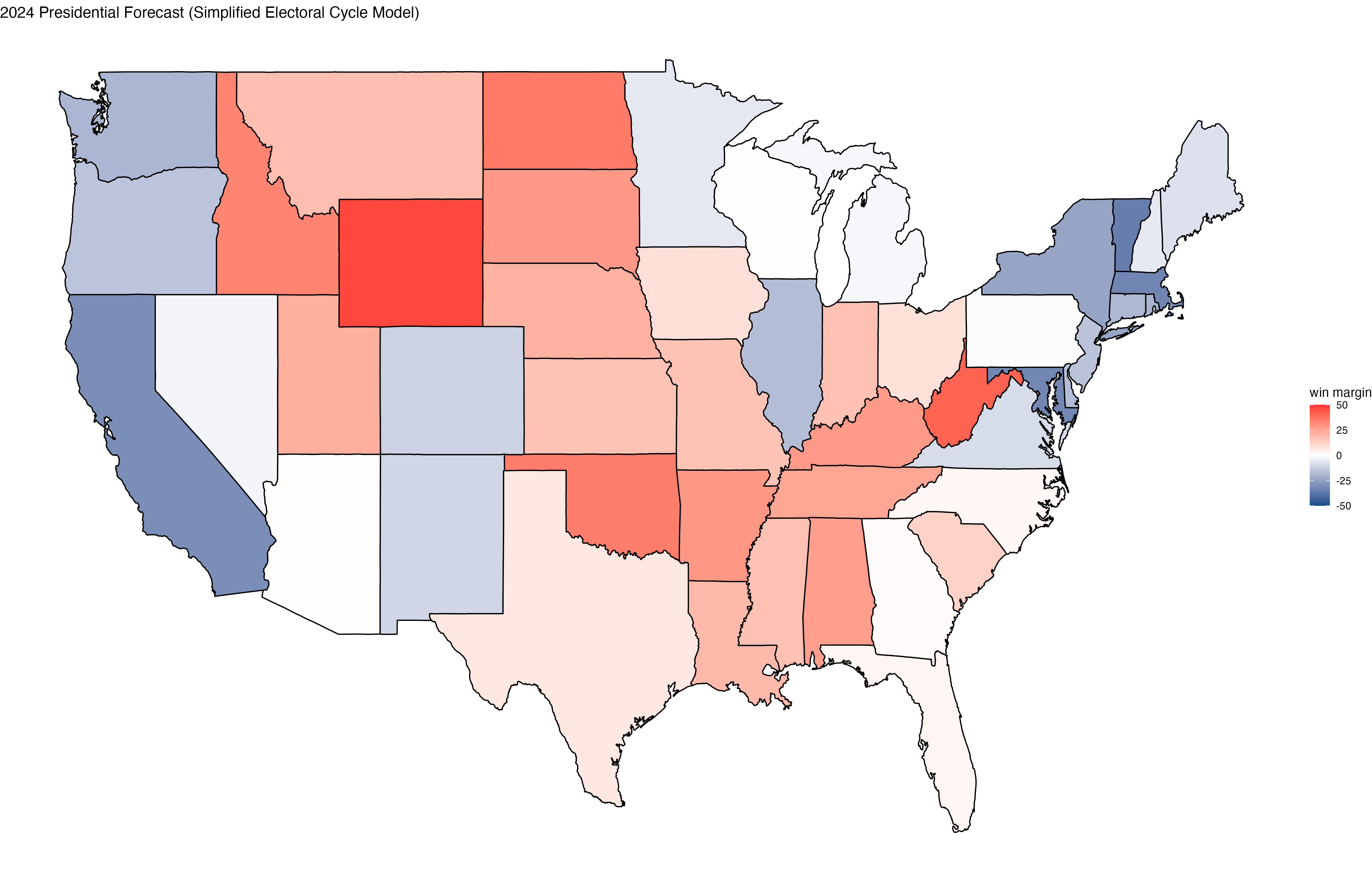
(Note that this map could be better labelled.)
If we go off this naïve, historically weighted model, Trump is expected to win a number of key battleground states: Arizona (+0.7%), Georgia (+1.15%), North Carolina (+2.0%), Florida (+2.9%), and Ohio (+8.5%). On the other hand, Harris is favored to win a fair share of battleground states including Wisconsin (+0.3%), Pennsylvannia (+0.7%), Michigan (+2.1%), Nevada (+2.5%), New Hampshire (+5.7%), Minnesota (+5.9%), and Maine (+7.8%).
Altogether, that spells out 276 EV for Harris and 262 EV for Trump in November.
Prediction 2: using past election returns and OLS.
We can also estimate simple bivariate and multivariate linear regressions using past electoral cycle returns. The first model uses vote share from the previous electoral cycle (2020) to predict the 2024 vote in each state using simple OLS as follows:
presvoteshare2024_i = beta_0 + beta_1*(presvoteshare2020_i)
The second model uses vote share from both 2020 and 2016 to predict the vote share in 2024 using multivariate OLS:
presvoteshare2024_i = beta_0 + beta_1*(presvoteshare2020_i) + beta_2*(presvoteshare2016_i)
Using these models, I obtained the following Electoral College vote predictions:
| Predictor Type | Harris | Trump |
|---|---|---|
| One Lagged Cycle Predictor | 226 | 312 |
| Two Lagged Cycle Predictors | 247 | 291 |
These predictions are quite a bit different than those obtained from Norpoth’s electoral cycle model. Why might that be?
Well, for one, the weights (coefficients) multiplying the lagged vote share variables will be different due to the fact that they were estimated directly from the data and come from a longer time period. We may or may not want to use all possible years in our prediction models (more on this later).
Second, the utility of including an intercept in these models is somewhat dubious;1 for example, if the vote for the GOP candidate in a state is 0 in 2020, we might reasonable expect the vote for the GOP candidate in a state in 2024 to be 0 as well. Including an intercept estimated from a model that pools states together may result in dramatically different predictions than models that only estimate 2024 vote using a weigthed sum of 2020 and 2016 votes.
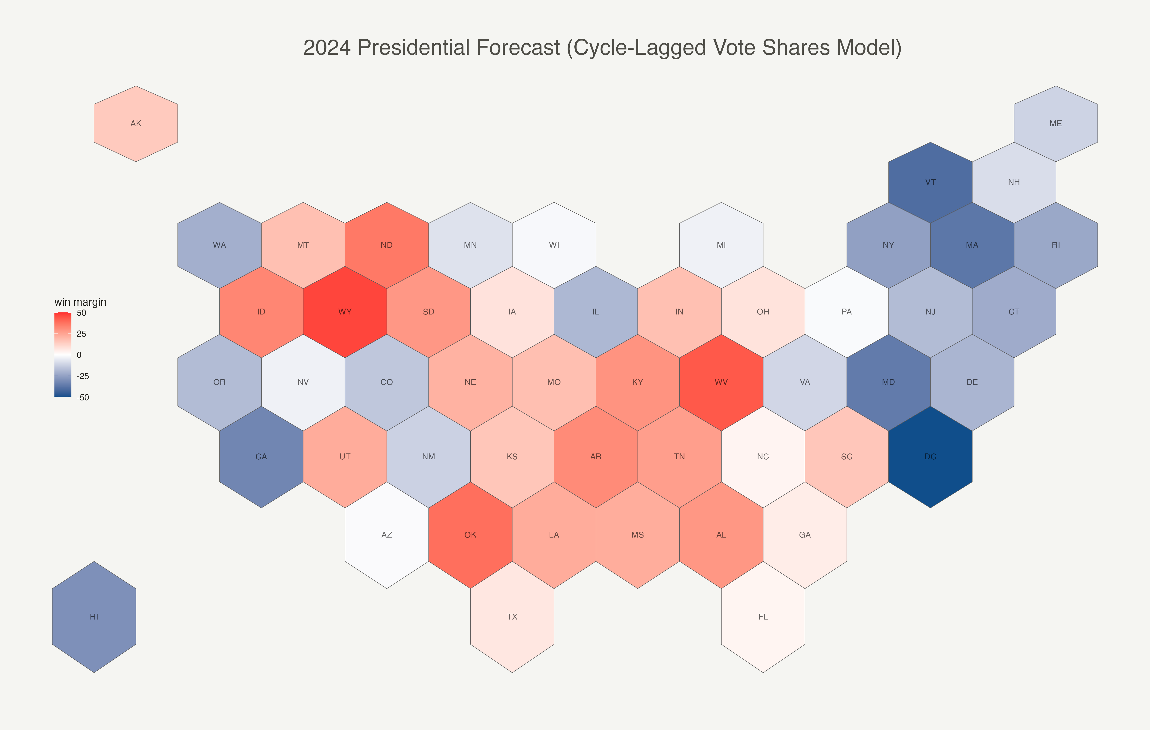
For our final introductory prediction techinque will use the two lagged cycle prediction model without an intercept and estimated separately for each state. This model predicts 287 EV for Harris and 251 EV for Trump in November.
Interestingly, this model only differs in terms of final prediction with respect to one swing state, Arizona, compared to Norpoth’s model. My state-level model predicts a Harris victory in Arizona. The model predictions are visualized below using a hex grid map of all US states and DC.